
Optimise your ROS snap – Part 1

gbeuzeboc
on 6 April 2023
Do you want to optimise the performance of your ROS snap? We reduced the size of the installed Gazebo snap by 95%!
This is how you can do it for your snap.
Welcome to Part 1 of the “optimise your ROS snap” blog series. This series of 6 blogs will show the tools and methodologies to measure and improve the performance of a snap. Throughout the series, we will use the Gazebo snap as an example to demonstrate how to optimise ROS snap.
Part 2 of this series will present the optimisations already present in our Gazebo snap.
While ROS snaps can be GUIs and desktop tools, they can also be the embedded software for robots. On a desktop, the user expects the application to start fast and not encumber the disk. On a robot, while we also expect the application to startup quickly, the bandwidth and storage accessible to the robot might certainly be limited. ROS snaps being C++ and Python applications and having tons of dependencies all included in our snap, they can quickly become quite heavy and sometimes long to launch. Our ROS snaps must be optimised!
In this blog post series, we will see the most common ways to improve our ROS snap in terms of space but also start-up time. Then we will explore what other less common optimisations can be done to improve our ROS snaps even more. Note that most of these tips also apply to non-ROS snaps. We will implement these optimisations on the Gazebo snap, benchmark every one of them and discuss their pros and cons. Later, we can decide what optimisation we want to apply to our ROS snap.
The Gazebo snap
It has been a few months since the Gazebo snap was announced and made available on the Snap Store. Back then, we published a blog post to demonstrate the possibilities with the snap. The snap code is available on GitHub and currently covers the Citadel release and ROS 2 Foxy.
This post assumes familiarity with snaps for ROS, as we are going to enter nitty-gritty details. If that’s not the case, we can take a look at the online documentation, the developer guide and our previous posts.
Benchmark tools and methodologies
Before doing any kind of optimisation we must be able to measure. We need a reproducible way to measure the impact of our optimisation in terms of size as well as in terms of time. In the next paragraphs, we are going to define our benchmarking methods.
Size
Since snaps bundle all their dependencies, they can quickly become large and take a lot of space on our system. Delivering updates or install in a bandwidth limited environment or on a disk space limited device can be challenging. This is why snap size is a metric that can’t be overlooked.
In terms of size, the benchmarking is going to be rather simple. We will simply report the size of the generated .snap file as well as the size of the installation directory. To measure the size of the current installation of our snap, we will use the following:
du -Dsh /snap/gazebo/currentTime
When running an application, we expect it to start as fast as possible. If an application takes too long to start, we might avoid using it. It could also interfere with the orchestration of other services and increase the downtime of our devices. For these reasons, it is important to keep track of time as a metric to improve performance.
In terms of time to launch the application, the benchmarking will be more complicated. Gazebo is mainly used as a graphic application. The performances of a graphic application can have different meaning. In the following sections, we will describe what exactly we are going to measure, as well as our methodology to create consistent benchmarks.
Start timing
Before explaining how we will be measuring the start timing, we should remember that snaps’ start-up time is different between a “cold” and a ”warm” start.
When talking about “cold start”, we mean launching the application without any libraries loaded into memory. Essentially, running Gazebo right after a boot. Such a cold start is very similar to the fresh installation start.
The fresh installation start can be easily reproduced by purging the previously installed snap with the command:
sudo snap remove --purge gazeboThis way, no libraries or files will be cached, and we will simulate the worst-case scenario.
Conversely, a warm start represents the case where we relaunch an application that we already installed and launch. Libraries are potentially cached, and in the snap everything is decompressed. It’s the best case scenario.
Start timing script
In order to properly measure the time Gazebo takes to start, we will use a small script using xdotool to detect the Gazebo window and time how long it took from launching the command to the window appearance.
The script runs both a cold start and warm start, making sure that we emptied our system cache. Finally, the script will append the results of the experiment in a file giving for both cases the sum of total number of CPU-seconds that the process used directly (in user mode) and total number of CPU-seconds used by the system on behalf of the process (in kernel mode), in seconds to depend as little as possible on the load of the computer.
This script is inspired by the one demonstrated in the blog post: how-to-make-snaps-faster and is available on GitHub.
Runtime performance
The runtime performance of a ROS snap can be critical depending on our application. In the case of Gazebo, the faster Gazebo runs, the faster we can simulate different scenarios. A slow simulation would also slow down the development process. The same analogy will apply to our application. That is why we should consider the runtime performances as a metric.
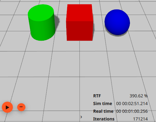
In order to measure the runtime performance of Gazebo, we will use the Real Time Factor (RTF). Since the RTF is very volatile (can change up to 200% in just a few seconds) we will compute the RTF on a one-minute averaging window. To do so, we will start the simulation paused, set the real time factor of the physic engine to 0 and run the simulation for approximately one minute. After that, we can pause and divide the simulation time by the real time available in the GUI. This provides us with a ratio to showcase the runtime performance of the snap.
Conclusion
Now, we have defined all the key metrics and why they are important. We also defined the tools and methodologies to optimise ROS snaps. We will be able to perform reliable measurements to properly evaluate the different optimisations that we will try in the next parts of this blog post series. All the measurements and tests will be done on the same computer (a ThinkPad laptop). Please note that we might measure different timings on another machine. The percentage of improvement is expected to be similar between machines.

Continue reading Part 2 of this series.
Talk to us today
Interested in running Ubuntu in your organisation?
Newsletter signup
Are you building a robot on top of Ubuntu and looking for a partner? Talk to us!

Related posts
TurtleBot3 OpenCR firmware update from a snap
The TurtleBot3 robot is a standard platform robot in the ROS community, and it’s a reference that Canonical knows well, since we’ve used it in our tutorials....
Canonical is now a platinum member in the Open Source Robotics Alliance
Ubuntu is the home of ROS. The very first ROS distribution, Box Turtle, launched on Ubuntu 8.04 LTS, Hardy Heron, and since then, Ubuntu and ROS have grown...
ROS Noetic is EOL – take action to maintain fleet security
As of May 2025, the Robot Operating System (ROS) Noetic Ninjemys officially reached its end of life (EOL). First released in 2020 as the final ROS (1)...